---
layout: post
title: Generative Adversarial Networks
---
We now move onto another family of generative models called generative adversarial networks (GANs). GANs are unique from all the other model families that we have seen so far, such as autoregressive models, VAEs, and normalizing flow models, because we do not train them using maximum likelihood.
Likelihood-free learning
==============
Why not? In fact, it is not so clear that better likelihood numbers necessarily correspond to higher sample quality. We know that the *optimal generative model* will give us the best sample quality and highest test log-likelihood. However, models with high test log-likelihoods can still yield poor samples, and vice versa. To see why, consider pathological cases in which our model is comprised almost entirely of noise, or our model simply memorizes the training set. Therefore, we turn to *likelihood-free training* with the hope that optimizing a different objective will allow us to disentangle our desiderata of obtaining high likelihoods as well as high-quality samples.
Recall that maximum likelihood required us to evaluate the likelihood of the data under our model $$p_\theta$$. A natural way to set up a likelihood-free objective is to consider the *two-sample test*, a statistical test that determines whether or not a finite set of samples from two distributions are from the same distribution *using only samples from $$P$$ and $$Q$$*. Concretely, given $$S_1 = \{\mathbf{x} \sim P\}$$ and $$S_2 = \{\mathbf{x} \sim Q\}$$, we compute a test statistic $$T$$ according to the difference in $$S_1$$ and $$S_2$$ that, when less than a threshold $$\alpha$$, accepts the null hypothesis that $$P = Q$$.
Analogously, we have in our generative modeling setup access to our training set $$S_1 = \mathcal{D} = \{\mathbf{x} \sim p_{\textrm{data}} \}$$ and $$S_2 = \{\mathbf{x} \sim p_{\theta} \}$$. The key idea is to train the model to minimize a *two-sample test objective* between $$S_1$$ and $$S_2$$. But this objective becomes extremely difficult to work with in high dimensions, so we choose to optimize a surrogate objective that instead *maximizes some distance* between $$S_1$$ and $$S_2$$.
GAN Objective
==============
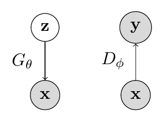
We thus arrive at the generative adversarial network formulation. There are two components in a GAN: (1) a generator and (2) a discriminator. The generator $$G_\theta$$ is a directed latent variable model that deterministically generates samples $$\mathbf{x}$$ from $$\mathbf{z}$$, and the discriminator $$D_\phi$$ is a function whose job is to distinguish samples from the real dataset and the generator. The image below is a graphical model of $$G_\theta$$ and $$D_\phi$$. $$\mathbf{x}$$ denotes samples (either from data or generator), $$\mathbf{z}$$ denotes our noise vector, and $$\mathbf{y}$$ denotes the discriminator's prediction about $$\mathbf{x}$$.
The generator and discriminator both play a two player minimax game, where the generator minimizes a two-sample test objective ($$p_{\textrm{data}} = p_\theta$$) and the discriminator maximizes the objective ($$p_{\textrm{data}} \neq p_\theta$$). Intuitively, the generator tries to fool the discriminator to the best of its ability by generating samples that look indistinguishable from $$p_{\textrm{data}}$$.
Formally, the GAN objective can be written as:
{% math %}
\min_{\theta} \max_{\phi} V(G_\theta, D_\phi) = \mathbb{E}_{\mathbf{x} \sim \textbf{p}_{\textrm{data}}}[\log D_\phi(\textbf{x})] +
\mathbb{E}_{\mathbf{z} \sim p(\textbf{z})}[\log (1-D_\phi(G_\theta(\textbf{z})))]
{% endmath %}
Let's unpack this expression. We know that the discriminator is maximizing this function with respect to its parameters $$\phi$$, where given a fixed generator $$G_\theta$$ it is performing binary classification: it assigns probability 1 to data points from the training set $$\mathbf{x} \sim p_{\textrm{data}}$$, and assigns probability 0 to generated samples $$\mathbf{x} \sim p_G$$. In this setup, the optimal discriminator is:
{% math %}
D^*_{G}(\mathbf{x}) = \frac{p_{\textrm{data}}(\mathbf{x})}{p_{\textrm{data}}(\mathbf{x}) + p_G(\mathbf{x})}
{% endmath %}
On the other hand, the generator minimizes this objective for a fixed discriminator $$D_\phi$$. And after performing some algebra, plugging in the optimal discriminator $$D^*_G(\cdot)$$ into the overall objective $$V(G_\theta, D^*_G(\mathbf{x}))$$ gives us:
{% math %}
2D_{\textrm{JSD}}[p_{\textrm{data}}, p_G] - \log 4
{% endmath %}
The $$D_{\textrm{JSD}}$$ term is the *Jenson-Shannon Divergence*, which is also known as the symmetric form of the KL divergence:
{% math %}
D_{\textrm{JSD}}[p, q] = \frac{1}{2} \left( D_{\textrm{KL}}\left[p, \frac{p+q}{2} \right] + D_{\textrm{KL}}\left[q, \frac{p+q}{2} \right] \right)
{% endmath %}
The JSD satisfies all properties of the KL, and has the additional perk that $$D_{\textrm{JSD}}[p,q] = D_{\textrm{JSD}}[q,p]$$. With this distance metric, the optimal generator for the GAN objective becomes $$p_G = p_{\textrm{data}}$$, and the optimal objective value that we can achieve with optimal generators and discriminators $$G^*(\cdot)$$ and $$D^*_{G^*}(\mathbf{x})$$ is $$-\log 4$$.
GAN training algorithm
==============
Thus, the way in which we train a GAN is as follows:
For epochs $$1, \ldots, N$$ do:
1. Sample minibatch of size $$m$$ from data: $$\mathbf{x}^{(1)}, \ldots, \mathbf{x}^{(m)} \sim \mathcal{D}$$
2. Sample minibatch of size $$m$$ of noise: $$\mathbf{z}^{(1)}, \ldots, \mathbf{z}^{(m)} \sim p_z$$
3. Take a gradient *descent* step on the generator parameters $$\theta$$:
{% math %}
\triangledown_\theta V(G_\theta, D_\phi) = \frac{1}{m} \triangledown_\theta \sum_{i=1}^m \log \left(1 - D_\phi(G_\theta(\mathbf{z}^{(i)})) \right)
{% endmath %}
4. Take a gradient *ascent* step on the discriminator parameters $$\phi$$:
{% math %}
\triangledown_\phi V(G_\theta, D_\phi) = \frac{1}{m} \triangledown_\phi \sum_{i=1}^m \left[\log D_\phi(\mathbf{x}^{(i)}) + \log (1 - D_\phi(G_\theta(\mathbf{z}^{(i)}))) \right]
{% endmath %}
Challenges
==============
Although GANs have been successfully applied to several domains and tasks, working with them in practice is challenging because of their: (1) unstable optimization procedure, (2) potential for mode collapse, (3) difficulty in evaluation.
During optimization, the generator and discriminator loss often continue to oscillate without converging to a clear stopping point. Due to the lack of a robust stopping criteria, it is difficult to know when exactly the GAN has finished training. Additionally, the generator of a GAN can often get stuck producing one of a few types of samples over and over again (mode collapse). Most fixes to these challenges are empirically driven, and there has been a significant amount of work put into developing new architectures, regularization schemes, and noise perturbations in an attempt to circumvent these issues. Soumith Chintala has a nice [link](https://github.com/soumith/ganhacks) outlining various tricks of the trade to stabilize GAN training.
Selected GANs
==============
Next, we focus our attention to a few select types of GAN architectures and explore them in more detail.
### f-GAN
The [f-GAN](https://arxiv.org/abs/1606.00709) optimizes the variant of the two-sample test objective that we have discussed so far, but using a very general notion of distance: the $$f divergence$$. Given two densities $$p$$ and $$q$$, the $$f$$-divergence can be written as:
{% math %}
D_f(p,q) = \mathbb{E}_{\mathbf{x}\sim q}\left[f \left(\frac{p(\mathbf{x})}{q(\mathbf{x})} \right) \right]
{% endmath %}
where $$f$$ is any convex[^1], lower-semicontinuous[^2] function with $$f(1) = 0$$. Several of the distance "metrics" that we have seen so far fall under the class of f-divergences, such as KL, Jenson-Shannon, and total variation.
To set up the f-GAN objective, we borrow two commonly used tools from convex optimization[^3]: the Fenchel conjugate and duality. Specifically, we obtain a lower bound to any f-divergence via its Fenchel conjugate:
{% math %}
D_f(p,q) \geq \sup_{T \in \mathcal{T}} \left(\mathbb{E}_{x \sim p}[T(\mathbf{x})] - \mathbb{E}_{x \sim q}[f^*(T(\mathbf{x}))] \right)
{% endmath %}
Therefore we can choose any f-divergence that we desire, let $$p = p_{\textrm{data}}$$ and $$q = p_G$$, parameterize $$T$$ by $$\phi$$ and $$G$$ by $$\theta$$, and obtain the following fGAN objective:
{% math %}
\min_\theta \max_\phi F(\theta,\phi) = \mathbb{E}_{x \sim p_{\textrm{data}}}[T_\phi(\mathbf{x})] - \mathbb{E}_{x \sim p_{G_\theta}}[f^*(T_\phi(\mathbf{x}))]
{% endmath %}
Intuitively, we can think about this objective as the generator trying to minimize the divergence estimate, while the discriminator tries to tighten the lower bound.
### BiGAN
We won't worry too much about the [BiGAN](https://arxiv.org/abs/1605.09782) in these notes. However, we can think about this model as one that allows us to infer latent representations even within a GAN framework.
### CycleGAN
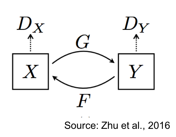
[CycleGAN](https://arxiv.org/abs/1703.10593) is a type of GAN that allows us to do unsupervised image-to-image translation, from two domains $$\mathcal{X} \leftrightarrow \mathcal{Y}$$.
Specifically, we learn two conditional generative models: $$G: \mathcal{X} \leftrightarrow \mathcal{Y}$$ and $$F: \mathcal{Y} \leftrightarrow \mathcal{X}$$. There is a discriminator $$D_\mathcal{Y}$$ associated with $$G$$ that compares the true $$Y$$ with the generated samples $$\hat{Y} = G(X)$$. Similarly, there is another discriminator $$D_\mathcal{X}$$ associated with $$F$$ that compares the true $$X$$ with the generated samples $$\hat{X} = F(Y)$$. The figure below illustrates the CycleGAN setup:
CycleGAN enforces a property known as *cycle consistency*, which states that if we can go from $$X$$ to $$\hat{Y}$$ via $$G$$, then we should also be able to go from $$\hat{Y}$$ to $$X$$ via $$F$$. The overall loss function can be written as:
{% math %}
\min_{F, G, D_\mathcal{X}, D_\mathcal{Y}} \mathcal{L}_{GAN}(G, D_\mathcal{Y}, X, Y) + \mathcal{L}_{GAN}(F, D_\mathcal{X}, X, Y) + \lambda \left(\mathbb{E}_X [||F(G(X)) - X||_1] + \mathbb{E}_Y [||G(F(Y)) - Y||_1] \right)
{% endmath %}
Footnotes
==============
[^1]: In this context, convex means a line joining any two points that lies above the function.
[^2]: The function value at any point $$\mathbf{x}_0$$ is close to or greater than $$f(\mathbf{x}_0)$$.
[^3]: This [book](http://web.stanford.edu/~boyd/cvxbook/) is an excellent resource to learn more about these topics.